Tutorial | Poisson Equation

Nonlinear Poisson Equation & Membrane Poisson

HeNeos

3 min readJun 4, 2023

Today, I want to explain a bit about how to solve one of the simplest and fundamental equations in PDE.

Poisson Equation

\begin{aligned}
-\nabla \cdot (q(u)\nabla u) = f
\end{aligned}

Here, the coefficient q(u) makes the equation nonlinear.

Applying the identity ∇ ⋅ (uv) = (∇ u)v + u⋅ ∇ v

\begin{aligned}
-\int_{\Omega} (\nabla \cdot (q(u)\nabla u)) v\,\mathrm{d}x &= \int_{\Omega} (q(u)\nabla u) \cdot \nabla v \, \mathrm{d} x - \int_{\Omega} \nabla\cdot (q(u)\nabla u) v \,\mathrm{d}x\cr
&= \int_{\Omega} f v\,\mathrm{d}x\cr
\text{Divergence theorem:} &\cr
&= \int_{\Omega} (q(u)\nabla u) \cdot \nabla v \, \mathrm{d} x - \int_{\partial \Omega} \mathrm{n}\cdot (q(u)\nabla u) v \,\mathrm{d}s
\end{aligned}

Applying weak form transformation: ∀ v ∈ 𝜕𝛺∶ v = 0

\begin{aligned}
&\int_{\Omega} (q(u)\nabla u) \cdot \nabla v \,\mathrm{d}x = \int_{\Omega} f v\,\mathrm{d}x\cr
F(u, v) &= \int_{\Omega} (q(u)\nabla u \cdot \nabla v - fv)\,\mathrm{d}x
\end{aligned}

Now, for the variational form:

\begin{aligned}
a(u,v) &= L(v)\cr
&= \int_{\Omega} (q(u)\nabla u) \cdot \nabla v \,\mathrm{d}x
\end{aligned}

and L(u,v) = ∫_𝛺 f v dx

V = FunctionSpace(mesh, 'P', 1)

u_D = Expression(u_ccode, degree=2)
bc = DirichletBC(V, u_D, boundary)

u = Function(V)
v = TestFunction(V)
f = Expression(f_ccode, degree=1)
F = q(u)*dot(grad(u), grad(v))*dx - f*v*dx

solve(F == 0, u, bc)

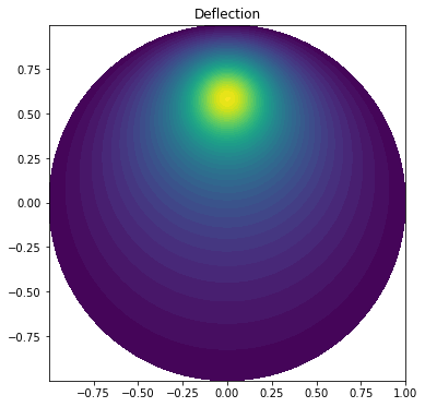
Membrane Poisson Equation

We want to compute the deflection D(x,y) of a two-dimensional, circular membrane of radius R, subject to a load p over the membrane. The appropriate PDE model is:

\begin{aligned}
-T\nabla^{2}D = p \quad \text{in}\; \Omega = \lbrace (x,y) \big\vert x^{2}+y^{2} \leq R \rbrace
\end{aligned}

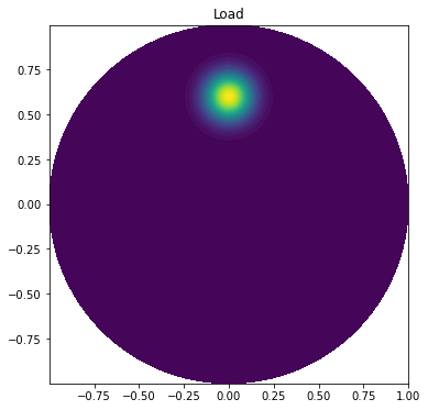
Here, T is the tension in the membrane (constant), and p is the external pressure load. The bounday of the membrane has no deflection, implying D = 0 as a boundary condition. A localized load can be modeled as a Gaussian function:

\begin{aligned}
p(x,y) = \frac{A}{2\pi\sigma} \exp\bigg( -\frac{1}{2}\Big(\frac{x-x_{0}}{\sigma}\Big)^{2} - \frac{1}{2} \Big(\frac{y-y_{0}}{\sigma}\Big)^{2} \bigg)
\end{aligned}

The parameter A is the amplitude of the pressure, (x₀, y₀) the localization of the maximum point of the load, and 𝜎 the “width” of p. We will take the center (x₀, y₀) of the pressure to be (0, R₀) for some 0<R₀<R.

\begin{aligned}
\nabla^{2} w = 4 \exp \big( -\beta^{2}(x^{2} + (y-R_{0})^{2}) \big), \quad (x,y) \in \Omega
\end{aligned}

Applying the identity ∇ ⋅ (uv) = (∇ u)v + u ⋅ ∇ v:

\begin{aligned}
-\int_{\Omega} (\nabla^{2} w) v\,\mathrm{d}x &= \int_{\Omega} \nabla w \cdot \nabla v \, \mathrm{d} x - \int_{\Omega} \nabla\cdot (\nabla w) v \,\mathrm{d}x\cr
&= \int_{\Omega} 4\exp(-\beta^{2}(x^{2}+(y-R_{0})^{2})) v\,\mathrm{d}x\cr
\text{Divergence theorem:}& \cr
&= \int_{\Omega} \nabla w \cdot \nabla v \, \mathrm{d} x - \int_{\partial \Omega} \mathrm{n}\cdot (\nabla w) v \,\mathrm{d}s
\end{aligned}

Applying weak form transformation ∀ v ∈ 𝜕𝛺, v = 0:

\begin{aligned}
\int_{\Omega} \nabla w \cdot \nabla v \,\mathrm{d}x = \int_{\Omega} 4\exp(-\beta^{2}(x^{2}+(y-R_{0})^{2})) v\,\mathrm{d}x
\end{aligned}

Now, for the variational form:

\begin{aligned}
a(u,v) &= L(v)\cr
&= \int_{\Omega} \nabla w \cdot \nabla v \,\mathrm{d}x\cr
L(u,v) &= \int_{\Omega} 4\exp(-\beta^{2}(x^{2}+(y-R_{0})^{2})) v\,\mathrm{d}x
\end{aligned}

# Define boundary condition
w_D = Constant(0) #w = 0 on boundaries

def boundary(x, on_boundary):
    return on_boundary

bc = DirichletBC(V, w_D, boundary)

# Define load
beta = 8
R0 = 0.6
p = Expression('4*exp(-pow(beta, 2)*(pow(x[0], 2) + pow(x[1] - R0, 2)))', degree=1, beta=beta, R0=R0)

# Define variational problem
w = TrialFunction(V)
v = TestFunction(V)
a = dot(grad(w), grad(v))*dx
L = p*v*dx

# Solve
w = Function(V)
solve(a == L, w, bc)